Graphical representation of functions

.6 Graphical representation of functions

Diagrams are very helpful in solving many mathematical problems involving functions. They are especially helpful in solving optimization problems, which occur throughout economic theory. Learning how to graphically represent functions will help enormously in understanding the material in this tutorial.

Functions of a single variable

A function of a single variable is most usefully represented by its graph.

Linear functions

A linear function of a single variable has the form

 f (x) = ax + b.

(Such a function is sometimes called "affine" rather than linear, the term "linear" being reserved by some mathematicians for functions of the form  f (x) = ax.) The graph of this function is a straight line with slope a; its value when x = 0 is b. Two examples are shown in the following figure.

Quadratic functions

A quadratic function of a single variable has the form

 f (x) = ax² + bx + c

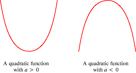
with a ≠ 0. The graph of such a function takes one of the two general forms shown in the following figure, depending on the sign of a.

The derivative of the function is zero when x = −b/2a, at which point the value of the function is c − b²/4a. The function may be written as

a(x + b/2a)² + c − b²/4a.

We can see from this expression that for any number z, the value of the function is the same at z − b/2a as it is at −z − b/2a. That is, the graph of the function is symmetric about a vertical line at x = −b/2a. The steepness of the graph depends on the parameters a and b: the derivative of the function at the point x is 2ax + b.

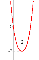
Example Sketch the graph of 2x2 − 8x + 6. The coefficient of x2 is positive, so the graph is U-shaped. The derivative is zero at x = 2, at which point the value of the function is −2. The value of the function at x= 0 is 6. The function is sketched in the following figure.

Reciprocal function

The function

 f (x) = c/x

has one of the forms shown in the following figure, depending on the sign of c. For c > 0 the graph is symmetric about the line with slope 1 through the origin; for c < 0 it is symmetric about the line with slope −1 through the origin.

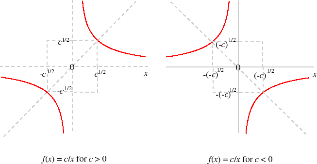
The curves in these diagrams are called "rectangular hyperbolae".

Exponential function

The function

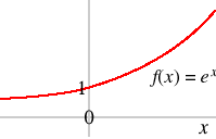
 f (x) = e^x

is positive for all values of x, has positive derivatives of every order, and takes the value 1 at x = 0. Its graph is shown in the following diagram.

Other functions

One way to get an idea of the shape of the graph of a arbitrary function of a single variable is to ask some plotting software on a computer to draw the graph. One such piece of software is available on the web. (Note that this software plots multiple functions: you enter a comma-separated list delimited by brackets---for example "[x^2, sin(x), exp(x)]".) If you don't have a computer handy, it is usually helpful to examine several characteristics of the function:

• the points (if any) at which its first derivative is zero
• its value at the points at which its first derivative is zero
• its value when x = 0
• the points at which its value is zero
• the behavior of its derivative.

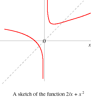
Example Sketch the function 2/x + x2. The derivative of this function is −2/x2 + 2x, which is zero when x = 1, at which point the second derivative is positive. The value of the function at x = 1 is 3. As xdecreases to 0 the value of the function increases without bound, and as x increases to 0 the value decreases without bound. The value of the function is zero when x = −21/3, and the derivative is negative for all negative values of x. Putting this information together we get the following figure.

Functions of two variables

The graph of a function of two variables is a surface in three dimensions. This surface may be represented in a perspective drawing on a piece of paper, but for many functions the drawing (a) is difficult to execute and (b) hides some features of the function---only parts are visible. Computer software allows one to construct such drawings easily, from many different viewpoints, solving both problems. But even so, another way of looking at a function of two variables is useful. This method, which involves the construction of a topographic map of the function, may easily be carried out by hand for many functions.

Level curves

Let  f  be a function of two variables, and c a constant. The set of pairs (x, y) such that

 f (x, y) = c

is called the level curve of  f  for the value c.

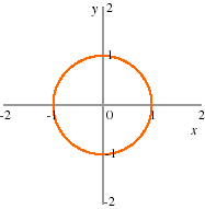
Example Let  f (x, y) = x2 + y2 for all (x, y). The level curve of  f  for the value 1 is the set of all pairs (x, y) such that x2 + y2 = 1, a circle of radius 1. This set is shown in the following figure.

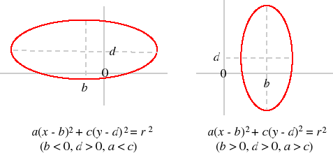
Example Let  f (x, y) = a(x − b)2 + c(y − d)2. Each level curve of this function is an ellipse centered at (b, d). If a = c the ellipse is a circle (as in the previous example). If a < c it is elongated horizontally; if a >c then the ellipse is elongated vertically. Examples are shown in the following figure.

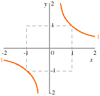
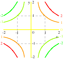
Example Let  f (x, y) = xy for all (x, y). The level curve of  f  for the value 1 is the set of all pairs (x, y) such that xy = 1, or, equivalently, y = 1/x. The part of this set for −2 ≤ x ≤ 2 and −2 ≤ y ≤ 2 is the union of the sets of points on the orange lines in the following figure.

By drawing the level curves of a function for various values, we construct a topographic map of the function that gives us a good picture of the nature of the function. If the values we choose are equally spaced (e.g. 1, 2, 3, or 10, 20, 30) then curves that are close indicate regions in which the rate of change of the function is large, whereas curves that are far apart indicate regions in which the rate of change of the function is small.

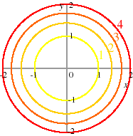
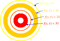
Example Let  f (x, y) = x2 + y2 for all (x, y). A collection of level curves of  f  is shown in the following figure. The number beside each curve is the value of the function to which it corresponds. We see that the graph of the function is a bowl with sides whose slopes increase as we move away from the center.

Example Let  f (x, y) = xy for all (x, y). A collection of level curves of  f  is shown in the following figure. The number beside each curve is the value of the function to which it corresponds. (The level curve for the value 0 consists of the axes.)

Note that a level curve is defined as a set, and indeed some level curves of some functions are not "curves" at all.

Consider, for example, the function  f  defined by  f (x, y) = 1 for all (x, y). (That is, the value of  f  is 1 for all values of x and y.) The level curve of this function for the value 2 is empty (there are no values of (x, y) such that  f (x, y) = 2) and the level curve for the value 1 is the set all all points (x, y).

In less extreme examples, some but not all level curves are sets. Consider a conicle terraced mountain, with terraces at heights of 10 and 30. Some level curves of this function are shown in the following figure. The level curves corresponding to heights of 10 and 30 are thick, whereas those corresponding to heights of 0 and 20 are not.

Contour lines on topographic maps of regions of the world are never thick because the earth is nowhere exactly flat (even in Manitoba).

Economists call the level curves of a utility function indifference curves and those of a production function isoquants.

Exercises